Excel Sum If With Multiple Criteria

FREE EXCEL VIDEO TRAINING/TUTORING > Trading Add-ins For excel > Convert Databases

IF YOU ARE USING 2007 or above, USE SUMIFS. FREE EXCEL HELP

There are many times that it become necessary to SUM cells based on multiple criteria. The examples below will show you 3 ways that this can be done. However, often the most efficient method is to use a Pivot Table If you are not familiar with Pivot Tables, I cannot stress enough how much easier spreadsheet life becomes once you are!

If you are not already aware, the Excel SUMIF formula/function can only check to see if specified cells meet one condition, e.g.

SUMIF Syntax

=SUMIF(range,criteria,sum_range)

=SUMIF(A1:A10,">20",B1:B10)

Which would SUM all numeric cells in the range B1:B20 where the corresponding row in A1:A10 was greater than 20. If we ommit the last optional argument (sum_range) the SUMIF would sum all cells in the range A1:A10 which are greater than 20, i.e.

=SUMIF(A1:A10,">20")

Note the criteria argument is in the form of a number, expression, or text that defines which cells will be summed. For example, criteria can be expressed as 20, "20", "=20", ">20", "North", "N*".

Ok, so if we need to sum a range of cells where corresponding cells (on the same row) meet 2, or more conditions we can no longer use the SUMIF. The formulas we can use, in order of their efficiency, are

1) DSUM Download advanced examples of DSUM
2) SUMPRODUCT
3) SUM with and IF function nested and entered as an array formula. See Array Formulas for details

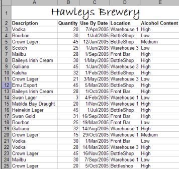
For all examples I will use the data as shown below. Where A2:E25 has been named: DataTable

DSUM

Adds the numbers in a column of a list, or database, that match criteria you specify. For example;

=DSUM(DataTable,B2,Criteria)

Would Sum all cells in B2:B25 that meet the criteria is the named range: Criteria (shown below)

The top row of the range: Criteria has exact copies of the headings in the range DataTable . The reference to cell B2 is telling the DSUM to sum the numbers in B2:B25 that meet the criteria. We could replace the reference to B2 with the text "Quantity", or the number 2 as the "Quantity" column is the second column in the table.

The criteria text "Bourbon" and "Vodka", under the criteria table heading "Description", tells DSUM that either "Bourbon" OR "Vodka" is a match. The same principle is used for the "Alcohol Content", i.e. "High" OR "Low". This is then seen by DSUM as an OR condition.

Note the repeat of the date under "Use By Date". This is needed when using more than 2 rows as the criteria as a blank cell is seen as a wildcard character. If we wanted to sum only data that lies between 2 dates, we would need have 2 "Use By Date" headings in our Criteria range and use: >7-Apr-2005 below one of these headings and <7-Jun-2005 under another. This is then seen by DSUM as an AND condition.

Download advanced examples of DSUM

SUMPRODUCT

Multiplies corresponding values in the given arrays, and returns the sum of those products=SUMPRODUCT((A3:A25="Vodka")*(C3:C25>VALUE("7-Apr-2005"))*(E3:E25="High")*(B3:B25))+SUMPRODUCT((A3:A25="Bourbon")*(C3:C25>VALUE("7-Apr-2005"))*(E3:E25="Low")*(B3:B25))

As with the first DSUM example, the above SUMPRODUCT example would sum all "Quantity" values where the corresponding "Use By Date" is greater than 7-Apr-2005, the "Description" is either "Vodka" OR "Bourbon" and the "Alcohol Content" is "High" OR "Low".

Note how range for each column of the table Start s at row 3 and not row 2. This is because the SUMPRODUCT has the result of each criteria check returned as TRUE (has a value of 1) or FALSE (has a value of 0). So, in the first row check (if we used row 2) it would look like;=SUMPRODUCT(0)*(0))*(0)*("Quantity"))+SUMPRODUCT((0)*(0)*(0)*("Quantity"))To read about this in detail, see our April edition of our free Excel Newsletter

The result of multiplying a text string is always #VALUE! This would cause the result of the SUMPRODUCT to return the #VALUE! error.

SUM and IF=SUM(IF(A2:A25="Bourbon",IF(C2:C25>VALUE("7-Apr-2005"),IF(E2:E25="Low",B2:B25)))+SUM(IF(A2:A25="Vodka",IF(C2:C25>VALUE("7-Apr-2005"),IF(E2:E25="High",B2:B25)))))

The above, does the same as the SUMPRODUCT example. However, this is an array formula and must be entered by pushing Ctrl+Shift+Enter

It is important to know that using the SUM and IF or the SUMPRODUCT over a large number of cells will cause a noticeable slow down in Excel's recalculation time. The DSUM is far more efficient in this regard. However, as stated at the very Start , a Pivot Table is better still when done correctly.

| | Helpful? Why Not Donate || ON SPECIAL! WHAT-IF ANALYSIS MANAGER - 30 DAY MONEY BACK - DOWNLOADS FOR EXCEL

Instant Download and Money Back Guarantee on Most Software

Microsoft Excel Training- From Beginner to Expert in 6 Hours/ EXCEL DASHBOARD REPORTS

Excel Trader Package Technical Analysis in Excel With $139.00 of FREE software!

Microsoft � and Microsoft Excel � are registered trademarks of Microsoft Corporation. OzGrid is in no way associated with Microsoft