Microsoft Excel Training- From Beginner to Expert in 6 Hours/ EXCEL DASHBOARD REPORTS

Excel: Alternate Row Colors/Color Banding

| | Information Helpful? Why Not Donate.

Color Every Second Row. Color all Odd/Even Rows

Got any Excel Questions? Free Excel Help

Alternate Row Colors/Color Banding

Now that Excel has Conditional Formatting (since Excel 97) we can use it to create an alternate row color for a table of data. This is often referred to as color banding and means that every second row should be filled with a specified color.

How to: Alternate Row Colors/Color Banding

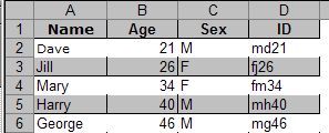
Let's say you have a table of data Starting in A1 and ending in D6. All you need to do is select the range A1:D6, Starting from A1, then go to Format>Conditional Formatting and choose "Formula is:" and then in the box to the right, type the formula as shown below;

=MOD(ROW(),2)

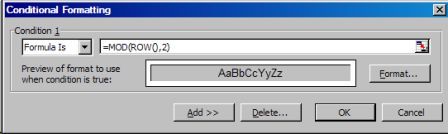
The MOD formula/function is used to return the remainder of a number (ROW()) after dividing it by a specified number, two (2) in this case.

The ROW formula/function will return the row number of the cell that houses it.

So the formula =MOD(ROW(),2) will only ever return 0 (zero) or 1. If you do not know already, 0 (zero) is equal to FALSE, while any number greater than 0 (zero) will equate to TRUE. When we use the "Formula is:" option of Conditional Formatting we must have a formula that returns only TRUE or FALSE. When TRUE, the format specified is applied. When FALSE, the format specified is not applied. With this in mind, we will return TRUE to all all rows where the row number divided by 2 equates to TRUE. Or, put another way, every second row.

Now click the "Format" button and choose your desired cell shading under "Patterns". Then "Ok" and "Ok" again.

Automatically Expand/Contract Alternate Row Colors/Color Banding

The simple method shown above is fine for a static table, but it will apply the format to all odd row numbers that do not yet have data. For example, we use the range A1:D6 but could use A1:D100 so that as our table has more data added the new row of data will be color coded automatically, while all unused rows will remain blank.

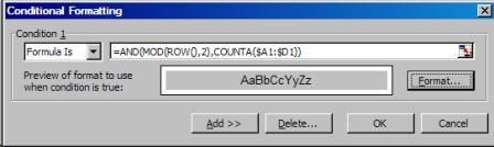
1) Select the A1:D100, Starting from A1.
2) Go to Format>Conditional Formatting and choose "Formula is:"
3) In the box to the right, type the formula as shown below;

=AND(MOD(ROW(),2),COUNTA($A1:$D1))

4) Click the "Format" button and choose your desired cell shading under "Patterns". Then "Ok" and "Ok" again.
Now only the used range of A1:D100 will have the alternate row color/banding.

Another way to do something very similar is to only include your used range in the initial selection, as we did at the Start , then go to Tools>Options-Edit and check the "Extend list formats and formulas". This will format new data added to the end of a list to match the format of the rest of the list. Formulas that are repeated in every row are also copied. To be extended, formats and formulas must appear in at least three of the five last rows preceding the new row.

How to: Alternate Row Colors/Color Banding 3D Effect

1) Select the A1:D100, Starting from A1.
2) Go to Format>Conditional Formatting and choose "Formula is:"
3) In the box to the right, type the formula as shown below;

=AND(MOD(ROW(),2),COUNTA($A1:$D1))

Note the absolute column and relative row reference: $A1:$D1
4) Click the "Format" button and choose your desired cell shading under "Patterns"
5) Click the "Border" page tab. Select Black under "Color", or Automatic if the default has not been changed. Now click on the solid black line at the bottom of the "Style" box. Click the bottom border of the box with the word "Text" in it and then click the right hand border.
6) Select White under "Color. Click the top border of the box with the word "Text" in it and then click the left hand border. It should look like below;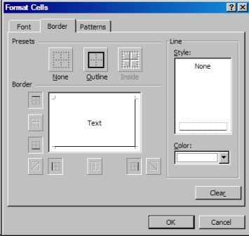

7) Click "Ok" then "Ok" again and you should see an effect like shown below;

Excel Dashboard Reports & Excel Dashboard Charts 50% Off Become an ExcelUser Affiliate & Earn Money

Special! Free Choice of Complete Excel Training Course OR Excel Add-ins Collection on all purchases totaling over $64.00. ALL purchases totaling over $150.00 gets you BOTH! Purchases MUST be made via this site. Send payment proof to [email protected] 31 days after purchase date.

Instant Download and Money Back Guarantee on Most Software

Microsoft Excel Training- From Beginner to Expert in 6 Hours/ EXCEL DASHBOARD REPORTS

Excel Trader Package Technical Analysis in Excel With $139.00 of FREE software!

Microsoft � and Microsoft Excel � are registered trademarks of Microsoft Corporation. OzGrid is in no way associated with Microsoft