Microsoft Excel Training- From Beginner to Expert in 6 Hours/ EXCEL DASHBOARD REPORTS

Excel Charts : Pie Chart Data Markers. Use Pie Chart as a Data Marker

| | Information Helpful? Why Not Donate.

Also see our huge range of Charting Software . Got a Excel Chart question? Use our FREE Excel Help

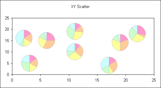
This is an example of using a pie chart as the custom marker within another chart.
You need to create a small pie chart that will be used as the custom marker. Format the chart area to have no fill pattern and no border. Format the slices as required.

To apply the chart as a data marker we first need to create a picture copy of it. This can be done manually within Excel. Hold the Shift key whilst selecting the pie chart.

Then whilst still holding the shift key click the Edit menu. Notice the appearance of a new menu item, Copy Picture.

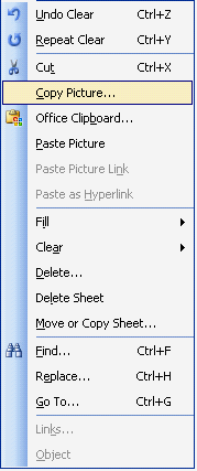
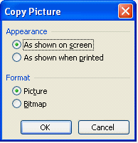
Selecting Copy Picture... will display a dialog that allows you to set some characteristics of the image that will be created on the clipboard.

On your xy scatter chart you need to click the data series and then click the appropriate data point. (See this tip for details of manually selecting individual chart elements ).

With the data point selected you can paste the pie chart using CTRL+V

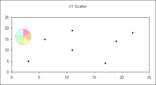
To do this for your whole chart you will need to change the data relating to the pie chart and the repeat the process of copying, selecting data point and pasting.

You can use VBA code to automate this process, which can be especially useful if the chart contains a lot of points or the data is changed at some point. As the pie data markers are static views of the data and are will not update with the data.

Sub PieMarkers()

    Dim chtMarker As Chart
    Dim chtMain As Chart
    Dim intPoint As Integer
    Dim rngRow As Range
    Dim lngPointIndex As Long

    Application.ScreenUpdating = False
     ' reference to pie chart
    Set chtMarker = ActiveSheet.ChartObjects("chtPieMarker").Chart
     ' reference to chart that pie markers will be applied to
    Set chtMain = ActiveSheet.ChartObjects(1).Chart

     ' pie chart data which will be processed by rows
    For Each rngRow In Range("F4:J11").Rows
         ' assign new values to pie chart
        chtMarker.SeriesCollection(1).Values = rngRow
         ' copy pie
        chtMarker.Parent.CopyPicture xlScreen, xlPicture
         ' paste to appropriate data point
        lngPointIndex = lngPointIndex + 1
        chtMain.SeriesCollection(1).Points(lngPointIndex).Paste
    Next

     ' release objects
    Set chtMarker = Nothing
    Set chtMain = Nothing
    Application.ScreenUpdating = False

End Sub

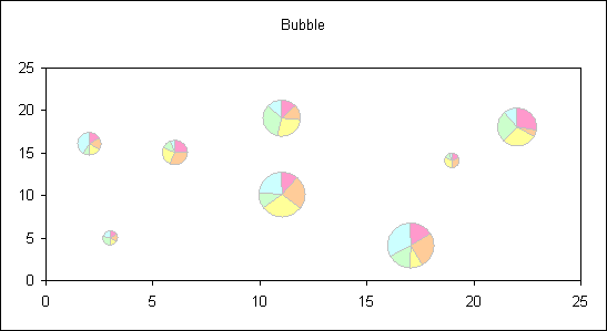
The same technique can be applied to a Bubble chart where the size of the pie is related to the bubble size value.

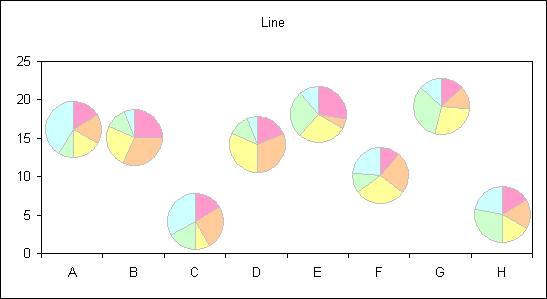
It can also be applied to a line chart.

The code and chart examples are contained within this workbook

Back to Excel Charts Index

Excel Dashboard Reports & Excel Dashboard Charts 50% Off Become an ExcelUser Affiliate & Earn Money

Special! Free Choice of Complete Excel Training Course OR Excel Add-ins Collection on all purchases totaling over $64.00. ALL purchases totaling over $150.00 gets you BOTH! Purchases MUST be made via this site. Send payment proof to [email protected] 31 days after purchase date.

Instant Download and Money Back Guarantee on Most Software

Microsoft Excel Training- From Beginner to Expert in 6 Hours/ EXCEL DASHBOARD REPORTS

Excel Trader Package Technical Analysis in Excel With $139.00 of FREE software!

Microsoft � and Microsoft Excel � are registered trademarks of Microsoft Corporation. OzGrid is in no way associated with Microsoft